Outputs
The quantities provided as outputs of hyperz have been already described
in the previous section. Here we report an example of the
.z_phot
file:
::::::::::::::
UBVRI.z_phot
::::::::::::::
| 1 |
0.600 |
0.442 |
77.86 |
2 |
29 |
1.0152 |
1.20 |
0.368E+03 |
0.541 |
0.647 |
... |
-18.90 |
1.380 |
0.00 |
| 2 |
3.020 |
0.032 |
96.89 |
1 |
28 |
0.7187 |
1.20 |
0.159E+05 |
2.791 |
3.051 |
... |
-26.11 |
5.200 |
93.50 |
| 3 |
0.200 |
0.687 |
60.05 |
1 |
30 |
1.4340 |
1.00 |
0.162E+03 |
0.000 |
0.277 |
... |
-14.03 |
1.940 |
0.02 |
| 4 |
3.200 |
0.071 |
99.09 |
5 |
27 |
0.5088 |
1.00 |
0.251E-06 |
2.899 |
3.332 |
... |
-22.94 |
2.600 |
37.71 |
| 5 |
4.400 |
0.019 |
99.64 |
1 |
7 |
0.0100 |
1.20 |
0.110E+02 |
3.967 |
4.669 |
... |
-22.61 |
2.800 |
87.07 |
As stated above, the format of this file is the following, ordered by columns:
(1) the identification number; (2) the photometric redshift primary solution;
(3) its  and (4) the corresponding probability; (5) the number of the spectral type
in the order of the spectra.param file; (6) the age record; (7)
the age in Gyr; (8) the absorption in the
  band to be applied at the best fit SED; (9) the normalization factor
  of equation 1 needed to minimize the
  ;
(10)-(11), (12)-(13) and (14)-(15) the limits of the confidence intervals
at 99%, 90% and 68%; (16) the weighted mean redshift
  ;
(17) the probability associated to
  (the columns 12 - 17 here are replaced by dots); (18) the absolute magnitude;
(19) the secondary peak of the probability function; (20) the probability
of the secondary solution.
One of the most considerable features of hyperz, is the possibility
of knowing the probability function  .
This characteristic allows us to describe in an accurate way the results
of different tests and to explore the relevance of secondary solutions
and then the degeneracy in the parameter space. Moreover, the function
 can be used to compute some cosmological quantities properly taking into
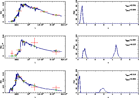
account the characteristics of the photometric redshift technique. Figure
7 shows an example of SED fitting and the
corresponding
 for three objects.
 |
Figure:Left: The best
fit SED (solid line), with superimposed the observed points with error
bars (vertical error bars correspond to photometric errors, horizontal
error bars represent the surface covered by the filter) and the fluxes
derived from the best fit SED (circles). Right: The probability
functions relative to for the three considered objects.
micol bolzonella
2000-12-10
![]() .
This characteristic allows us to describe in an accurate way the results
of different tests and to explore the relevance of secondary solutions
and then the degeneracy in the parameter space. Moreover, the function
.
This characteristic allows us to describe in an accurate way the results
of different tests and to explore the relevance of secondary solutions
and then the degeneracy in the parameter space. Moreover, the function![]() can be used to compute some cosmological quantities properly taking into
account the characteristics of the photometric redshift technique. Figure
7 shows an example of SED fitting and the
corresponding
can be used to compute some cosmological quantities properly taking into
account the characteristics of the photometric redshift technique. Figure
7 shows an example of SED fitting and the
corresponding![]() for three objects.
for three objects.
